Chapter 4. Data Management

The Open Geospatial Consortium (OGC) developed the Simple Features Access standard (SFA) to provide a model for geospatial data. It defines the fundamental spatial type of Geometry, along with operations which manipulate and transform geometry values to perform spatial analysis tasks. PostGIS implements the OGC Geometry model as the PostgreSQL data types geometry and geography.

Geometry is an abstract type. Geometry values belong to one of its concrete subtypes which represent various kinds and dimensions of geometric shapes. These include the atomic types Point, LineString, LinearRing and Polygon, and the collection types MultiPoint, MultiLineString, MultiPolygon and GeometryCollection. The Simple Features Access - Part 1: Common architecture v1.2.1 adds subtypes for the structures PolyhedralSurface, Triangle and TIN.

Geometry models shapes in the 2-dimensional Cartesian plane. The PolyhedralSurface, Triangle, and TIN types can also represent shapes in 3-dimensional space. The size and location of shapes are specified by their coordinates. Each coordinate has a X and Y ordinate value determining its location in the plane. Shapes are constructed from points or line segments, with points specified by a single coordinate, and line segments by two coordinates.

Coordinates may contain optional Z and M ordinate values. The Z ordinate is often used to represent elevation. The M ordinate contains a measure value, which may represent time or distance. If Z or M values are present in a geometry value, they must be defined for each point in the geometry. If a geometry has Z or M ordinates the coordinate dimension is 3D; if it has both Z and M the coordinate dimension is 4D.

Geometry values are associated with a spatial reference system indicating the coordinate system in which it is embedded. The spatial reference system is identified by the geometry SRID number. The units of the X and Y axes are determined by the spatial reference system. In planar reference systems the X and Y coordinates typically represent easting and northing, while in geodetic systems they represent longitude and latitude. SRID 0 represents an infinite Cartesian plane with no units assigned to its axes. See Section 4.5, “The SPATIAL_REF_SYS Table and Spatial Reference Systems”.

The geometry dimension is a property of geometry types. Point types have dimension 0, linear types have dimension 1, and polygonal types have dimension 2. Collections have the dimension of the maximum element dimension.

A geometry value may be empty. Empty values contain no vertices (for atomic geometry types) or no elements (for collections).

An important property of geometry values is their spatial extent or bounding box, which the OGC model calls envelope. This is the 2 or 3-dimensional box which encloses the coordinates of a geometry. It is an efficient way to represent a geometry's extent in coordinate space and to check whether two geometries interact.

The geometry model allows evaluating topological spatial relationships as described in Section 5.1.1, “Dimensionally Extended 9-Intersection Model”. To support this the concepts of interior, boundary and exterior are defined for each geometry type. Geometries are topologically closed, so they always contain their boundary. The boundary is a geometry of dimension one less than that of the geometry itself.

The OGC geometry model defines validity rules for each geometry type. These rules ensure that geometry values represents realistic situations (e.g. it is possible to specify a polygon with a hole lying outside the shell, but this makes no sense geometrically and is thus invalid). PostGIS also allows storing and manipulating invalid geometry values. This allows detecting and fixing them if needed. See Section 4.4, “Geometry Validation”

POINT (1 2)
POINT Z (1 2 3)
POINT ZM (1 2 3 4)

LINESTRING (1 2, 3 4, 5 6)

LINEARRING (0 0 0, 4 0 0, 4 4 0, 0 4 0, 0 0 0)

POLYGON ((0 0 0,4 0 0,4 4 0,0 4 0,0 0 0),(1 1 0,2 1 0,2 2 0,1 2 0,1 1 0))

MULTIPOINT ( (0 0), (1 2) )

MULTILINESTRING ( (0 0,1 1,1 2), (2 3,3 2,5 4) )

MULTIPOLYGON (((1 5, 5 5, 5 1, 1 1, 1 5)), ((6 5, 9 1, 6 1, 6 5)))

GEOMETRYCOLLECTION ( POINT(2 3), LINESTRING(2 3, 3 4))

POLYHEDRALSURFACE Z (
  ((0 0 0, 0 0 1, 0 1 1, 0 1 0, 0 0 0)),
  ((0 0 0, 0 1 0, 1 1 0, 1 0 0, 0 0 0)),
  ((0 0 0, 1 0 0, 1 0 1, 0 0 1, 0 0 0)),
  ((1 1 0, 1 1 1, 1 0 1, 1 0 0, 1 1 0)),
  ((0 1 0, 0 1 1, 1 1 1, 1 1 0, 0 1 0)),
  ((0 0 1, 1 0 1, 1 1 1, 0 1 1, 0 0 1)) )

TRIANGLE ((0 0, 0 9, 9 0, 0 0))

TIN Z ( ((0 0 0, 0 0 1, 0 1 0, 0 0 0)), ((0 0 0, 0 1 0, 1 1 0, 0 0 0)) )

The ISO/IEC 13249-3 SQL Multimedia - Spatial standard (SQL/MM) extends the OGC SFA to define Geometry subtypes containing curves with circular arcs. The SQL/MM types support 3DM, 3DZ and 4D coordinates.

	Todos as comparações de pontos flutuantes dentro da implementação SQL-MM são representadas com uma tolerância específica, atualmente 1E-8.

CIRCULARSTRING(0 0, 1 1, 1 0)

CIRCULARSTRING(0 0, 4 0, 4 4, 0 4, 0 0)

COMPOUNDCURVE( CIRCULARSTRING(0 0, 1 1, 1 0),(1 0, 0 1))

CURVEPOLYGON(
  CIRCULARSTRING(0 0, 4 0, 4 4, 0 4, 0 0),
  (1 1, 3 3, 3 1, 1 1) )

CURVEPOLYGON(
  COMPOUNDCURVE( CIRCULARSTRING(0 0,2 0, 2 1, 2 3, 4 3),
                 (4 3, 4 5, 1 4, 0 0)),
  CIRCULARSTRING(1.7 1, 1.4 0.4, 1.6 0.4, 1.6 0.5, 1.7 1) )

MULTICURVE( (0 0, 5 5), CIRCULARSTRING(4 0, 4 4, 8 4))

MULTISURFACE(
  CURVEPOLYGON(
    CIRCULARSTRING( 0 0, 4 0, 4 4, 0 4, 0 0),
    (1 1, 3 3, 3 1, 1 1)),
  ((10 10, 14 12, 11 10, 10 10), (11 11, 11.5 11, 11 11.5, 11 11)))

A especificação OpenGIS define dois caminhos padrão de expressar objetos espaciais: o Well-Known Text (WKT) e o Well-Known Binary (WKB). Ambos incluem informação sobre o tipo do objeto e as coordenadas que os formam.

A representação bem conhecida de texto do sistema de referência espacial. Um exemplo de uma representação WKT SRS é:

Input and output of WKT is provided by the functions ST_AsText and ST_GeomFromText:

text WKT = ST_AsText(geometry);
geometry = ST_GeomFromText(text WKT, SRID);

Por exemplo, uma declaração inserida válida para criar e inserir um objeto espacial OGC seria:

INSERT INTO geotable ( geom, name )
  VALUES ( ST_GeomFromText('POINT(-126.4 45.32)', 312), 'A Place');

Well-Known Binary (WKB) provides a portable, full-precision representation of spatial data as binary data (arrays of bytes). Examples of the WKB representations of spatial objects are:

Input and output of WKB is provided by the functions ST_AsBinary and ST_GeomFromWKB:

bytea WKB = ST_AsBinary(geometry);
geometry = ST_GeomFromWKB(bytea WKB, SRID);

Por exemplo, uma declaração inserida válida para criar e inserir um objeto espacial OGC seria:

INSERT INTO geotable ( geom, name )
  VALUES ( ST_GeomFromWKB('\x0101000000000000000000f03f000000000000f03f', 312), 'A Place');

OGC SFA specifications initially supported only 2D geometries, and the geometry SRID is not included in the input/output representations. The OGC SFA specification 1.2.1 (which aligns with the ISO 19125 standard) adds support for 3D (ZYZ) and measured (XYM and XYZM) coordinates, but still does not include the SRID value.

Because of these limitations PostGIS defined extended EWKB and EWKT formats. They provide 3D (XYZ and XYM) and 4D (XYZM) coordinate support and include SRID information. Including all geometry information allows PostGIS to use EWKB as the format of record (e.g. in DUMP files).

EWKB and EWKT are used for the "canonical forms" of PostGIS data objects. For input, the canonical form for binary data is EWKB, and for text data either EWKB or EWKT is accepted. This allows geometry values to be created by casting a text value in either HEXEWKB or EWKT to a geometry value using ::geometry. For output, the canonical form for binary is EWKB, and for text it is HEXEWKB (hex-encoded EWKB).

For example this statement creates a geometry by casting from an EWKT text value, and outputs it using the canonical form of HEXEWKB:

SELECT 'SRID=4;POINT(0 0)'::geometry;
  geometry
  ----------------------------------------------------
  01010000200400000000000000000000000000000000000000

PostGIS EWKT output has a few differences to OGC WKT:

EWKT avoids over-specifying dimensionality and the inconsistencies that can occur with the OGC/ISO format, such as:

	Os formatos estendidos do PostGIS estão atualmente superset de OGC (cada WKB/WKT válido é um EWKB/EWKT válido), mas isto pode airar no futuro, especificamente se OGC sai com um novo formato conflitando com nossas extensões. Assim, você NÃO DEVE confiar neste aspecto!

A seguir, exemplos das representações de textos (WKT) dos objetos espaciais das características:

Entrada/Saída destes formatos estão disponíveis usando as seguintes interfaces:

bytea EWKB = ST_AsEWKB(geometry);
text EWKT = ST_AsEWKT(geometry);
geometry = ST_GeomFromEWKB(bytea EWKB);
geometry = ST_GeomFromEWKT(text EWKT);

Por exemplo, uma declaração inserida válida para criar e inserir um objeto espacial seria:

INSERT INTO geotable ( geom, name )
  VALUES ( ST_GeomFromEWKT('SRID=312;POINTM(-126.4 45.32 15)'), 'A Place' )

You can create a table to store geography data using the CREATE TABLE SQL statement with a column of type geography. The following example creates a table with a geography column storing 2D LineStrings in the WGS84 geodetic coordinate system (SRID 4326):

CREATE TABLE global_points (
    id SERIAL PRIMARY KEY,
    name VARCHAR(64),
    location geography(POINT,4326)
  );

The geography type supports two optional type modifiers:

Examples of creating tables with geography columns:

Geography fields are registered in the geography_columns system view. You can query the geography_columns view and see that the table is listed:

SELECT * FROM geography_columns;

Criar um índice funciona da mesma forma que uma GEOMETRIA. O PostGIS irá notar que o tipo de coluna é GEOGRAFIA e criará um índice baseado em esfera apropriado em vez do de costume usado para GEOMETRIA.

-- Index the test table with a spherical index
CREATE INDEX global_points_gix ON global_points USING GIST ( location );

You can insert data into geography tables in the same way as geometry. Geometry data will autocast to the geography type if it has SRID 4326. The EWKT and EWKB formats can also be used to specify geography values.

-- Add some data into the test table
INSERT INTO global_points (name, location) VALUES ('Town', 'SRID=4326;POINT(-110 30)');
INSERT INTO global_points (name, location) VALUES ('Forest', 'SRID=4326;POINT(-109 29)');
INSERT INTO global_points (name, location) VALUES ('London', 'SRID=4326;POINT(0 49)');

Any geodetic (long/lat) spatial reference system listed in spatial_ref_sys table may be specified as a geography SRID. Non-geodetic coordinate systems raise an error if used.

-- NAD 83 lon/lat
SELECT 'SRID=4269;POINT(-123 34)'::geography;
                    geography
----------------------------------------------------
 0101000020AD1000000000000000C05EC00000000000004140

-- NAD27 lon/lat
SELECT 'SRID=4267;POINT(-123 34)'::geography;
                    geography
----------------------------------------------------
 0101000020AB1000000000000000C05EC00000000000004140

-- NAD83 UTM zone meters - gives an error since it is a meter-based planar projection
SELECT 'SRID=26910;POINT(-123 34)'::geography;

ERROR:  Only lon/lat coordinate systems are supported in geography.

As funções de consulta e medida usam unidades em metros. Então, os parâmetros de distância deveriam ser esperados em metros (ou metros quadrados para áreas).

-- A distance query using a 1000km tolerance
SELECT name FROM global_points WHERE ST_DWithin(location, 'SRID=4326;POINT(-110 29)'::geography, 1000000);

You can see the power of geography in action by calculating how close a plane flying a great circle route from Seattle to London (LINESTRING(-122.33 47.606, 0.0 51.5)) comes to Reykjavik (POINT(-21.96 64.15)) (map the route).

O tipo GEOGRAFIA calcula a verdadeira menor distância sobre a esfera entre Reykjavik e o grande caminho de voo circular entre Seattle e Londres.

-- Distance calculation using GEOGRAPHY
SELECT ST_Distance('LINESTRING(-122.33 47.606, 0.0 51.5)'::geography, 'POINT(-21.96 64.15)'::geography);
   st_distance
-----------------
 122235.23815667

Great Circle mapper A GEOMETRIA calcula a distância cartesiana insignificante entre Reykjavik e o caminho direto de Seattle para Londres marcado em um mapa. As unidades nominais do resultado podem ser chamadas de "graus", mas o resultado não corresponde a nenhuma diferença angular verdadeira entre os pontos, então, chamá-las de "graus" é incoerente.

-- Distance calculation using GEOMETRY
SELECT ST_Distance('LINESTRING(-122.33 47.606, 0.0 51.5)'::geometry, 'POINT(-21.96 64.15)'::geometry);
      st_distance
--------------------
 13.342271221453624

The geography data type allows you to store data in longitude/latitude coordinates, but at a cost: there are fewer functions defined on GEOGRAPHY than there are on GEOMETRY; those functions that are defined take more CPU time to execute.

O tipo que você escolheu deveria ser condicionado da área de trabalho esperada da aplicação que você está construindo. Seus dados irão abranger o globo ou uma grande área continental, ou é local para um estado, condado ou município?

Recorra a Section 13.11, “PostGIS Function Support Matrix” para uma comparação entre o que é suportado pela Geografia vs. Geometria. Para uma breve lista e descrição das funções da Geografia, recorra a Section 13.4, “PostGIS Geography Support Functions”

A simple geometry is one that has no anomalous geometric points, such as self intersection or self tangency.

Um POINT é herdado simple como um objeto geométrico 0-dimensional.

MULTIPOINTs são simple se nenhuma de duas coordenadas (POINTs) forem iguais (tenham o valor de coordenadas idêntico).

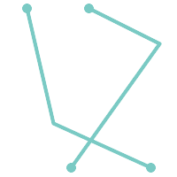
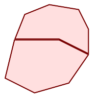
A LINESTRING is simple if it does not pass through the same point twice, except for the endpoints. If the endpoints of a simple LineString are identical it is called closed and referred to as a Linear Ring.

(a) and (c) are simple LINESTRINGs. (b) and (d) are not simple. (c) is a closed Linear Ring.

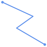
(a)	(b)
(c)	(d)

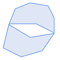
A MULTILINESTRING is simple only if all of its elements are simple and the only intersection between any two elements occurs at points that are on the boundaries of both elements.

(e) and (f) are simple MULTILINESTRINGs. (g) is not simple.

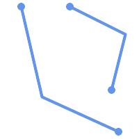
(e)

(f)

(g)

POLYGONs are formed from linear rings, so valid polygonal geometry is always simple.

To test if a geometry is simple use the ST_IsSimple function:

SELECT
   ST_IsSimple('LINESTRING(0 0, 100 100)') AS straight,
   ST_IsSimple('LINESTRING(0 0, 100 100, 100 0, 0 100)') AS crossing;

 straight | crossing
----------+----------
 t        | f

Generally, PostGIS functions do not require geometric arguments to be simple. Simplicity is primarily used as a basis for defining geometric validity. It is also a requirement for some kinds of spatial data models (for example, linear networks often disallow lines that cross). Multipoint and linear geometry can be made simple using ST_UnaryUnion.

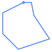
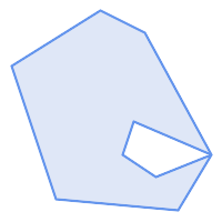
Geometry validity primarily applies to 2-dimensional geometries (POLYGONs and MULTIPOLYGONs) . Validity is defined by rules that allow polygonal geometry to model planar areas unambiguously.

A POLYGON is valid if:

(h) and (i) are valid POLYGONs. (j-m) are invalid. (j) can be represented as a valid MULTIPOLYGON.

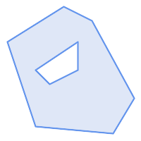
(h)	(i)	(j)
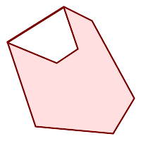
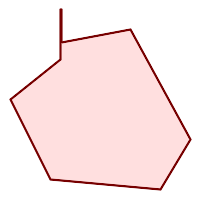
(k)	(l)	(m)

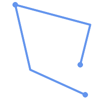
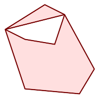
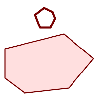
A MULTIPOLYGON is valid if:

(n) is a valid MULTIPOLYGON. (o) and (p) are invalid.

(n)

(o)

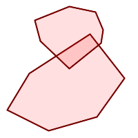
(p)

These rules mean that valid polygonal geometry is also simple.

For linear geometry the only validity rule is that LINESTRINGs must have at least two points and have non-zero length (or equivalently, have at least two distinct points.) Note that non-simple (self-intersecting) lines are valid.

SELECT
   ST_IsValid('LINESTRING(0 0, 1 1)') AS len_nonzero,
   ST_IsValid('LINESTRING(0 0, 0 0, 0 0)') AS len_zero,
   ST_IsValid('LINESTRING(10 10, 150 150, 180 50, 20 130)') AS self_int;

 len_nonzero | len_zero | self_int
-------------+----------+----------
 t           | f        | t

POINT and MULTIPOINT geometries have no validity rules.

PostGIS allows creating and storing both valid and invalid Geometry. This allows invalid geometry to be detected and flagged or fixed. There are also situations where the OGC validity rules are stricter than desired (examples of this are zero-length linestrings and polygons with inverted holes.)

Many of the functions provided by PostGIS rely on the assumption that geometry arguments are valid. For example, it does not make sense to calculate the area of a polygon that has a hole defined outside of the polygon, or to construct a polygon from a non-simple boundary line. Assuming valid geometric inputs allows functions to operate more efficiently, since they do not need to check for topological correctness. (Notable exceptions are that zero-length lines and polygons with inversions are generally handled correctly.) Also, most PostGIS functions produce valid geometry output if the inputs are valid. This allows PostGIS functions to be chained together safely.

If you encounter unexpected error messages when calling PostGIS functions (such as "GEOS Intersection() threw an error!"), you should first confirm that the function arguments are valid. If they are not, then consider using one of the techniques below to ensure the data you are processing is valid.

	If a function reports an error with valid inputs, then you may have found an error in either PostGIS or one of the libraries it uses, and you should report this to the PostGIS project. The same is true if a PostGIS function returns an invalid geometry for valid input.

To test if a geometry is valid use the ST_IsValid function:

SELECT ST_IsValid('POLYGON ((20 180, 180 180, 180 20, 20 20, 20 180))');
-----------------
 t

Information about the nature and location of an geometry invalidity are provided by the ST_IsValidDetail function:

SELECT valid, reason, ST_AsText(location) AS location
    FROM ST_IsValidDetail('POLYGON ((20 20, 120 190, 50 190, 170 50, 20 20))') AS t;

 valid |      reason       |                  location
-------+-------------------+---------------------------------------------
 f     | Self-intersection | POINT(91.51162790697674 141.56976744186045)

In some situations it is desirable to correct invalid geometry automatically. Use the ST_MakeValid function to do this. (ST_MakeValid is a case of a spatial function that does allow invalid input!)

By default, PostGIS does not check for validity when loading geometry, because validity testing can take a lot of CPU time for complex geometries. If you do not trust your data sources, you can enforce a validity check on your tables by adding a check constraint:

ALTER TABLE mytable
  ADD CONSTRAINT geometry_valid_check
        CHECK (ST_IsValid(geom));

The SPATIAL_REF_SYS table used by PostGIS is an OGC-compliant database table that defines the available spatial reference systems. It holds the numeric SRIDs and textual descriptions of the coordinate systems.

A tabela SPATIAL_REF_SYS de definição está como segue:

CREATE TABLE spatial_ref_sys (
  srid       INTEGER NOT NULL PRIMARY KEY,
  auth_name  VARCHAR(256),
  auth_srid  INTEGER,
  srtext     VARCHAR(2048),
  proj4text  VARCHAR(2048)
)

As opções da commandline são:

When retrieving spatial reference system definitions for use in transformations, PostGIS uses fhe following strategy:

The PostGIS spatial_ref_sys table contains over 3000 of the most common spatial reference system definitions that are handled by the PROJ projection library. But there are many coordinate systems that it does not contain. You can add SRS definitions to the table if you have the required information about the spatial reference system. Or, you can define your own custom spatial reference system if you are familiar with PROJ constructs. Keep in mind that most spatial reference systems are regional and have no meaning when used outside of the bounds they were intended for.

Uma ótima fonte para encontrar sistemas de referência espacial não definidos na configuração central é http://spatialreference.org/

Alguns dos sistemas de referência espacial mais comumente usados são: 4326 - WGS 84 Long Lat, 4269 - NAD 83 Long Lat, 3395 - WGS 84 World Mercator, 2163 - US National Atlas Equal Area, Spatial reference systems para cadaNAD 83, WGS 84 UTM zona - zonas UTM são as mais ideais para medição, mas só cobrem 6-graus regiões.

Vários estados dos EUA no sistema de referência espacial (em metros ou pés) - normalmente um ou 2 existem por estado. A maioria dos que estão em metros estão no centro, mas muitos dos que estão em pés ou foram criados por ESRI precisarão de spatialreference.org.

You can even define non-Earth-based coordinate systems, such as Mars 2000 This Mars coordinate system is non-planar (it's in degrees spheroidal), but you can use it with the geography type to obtain length and proximity measurements in meters instead of degrees.

Here is an example of loading a custom coordinate system using an unassigned SRID and the PROJ definition for a US-centric Lambert Conformal projection:

INSERT INTO spatial_ref_sys (srid, proj4text)
VALUES ( 990000,
  '+proj=lcc  +lon_0=-95 +lat_0=25 +lat_1=25 +lat_2=25 +x_0=0 +y_0=0 +datum=WGS84 +units=m +no_defs'
);

You can create a table to store geometry data using the CREATE TABLE SQL statement with a column of type geometry. The following example creates a table with a geometry column storing 2D (XY) LineStrings in the BC-Albers coordinate system (SRID 3005):

CREATE TABLE roads (
    id SERIAL PRIMARY KEY,
    name VARCHAR(64),
    geom geometry(LINESTRING,3005)
  );

The geometry type supports two optional type modifiers:

ALTER TABLE roads ADD COLUMN geom2 geometry(LINESTRINGZ,4326);